Taking Advantage of Sparsity in the ALS-WR Algorithm
I was interested in learning how to put together a recommender system for fun and practice. Since the Alternating-Least-Squares with Weighted-\(\lambda\)-Regularization (ALS-WR) algorithm seems to be a popular algorithm for recommender systems, I decided to give it a shot. It was developed for the Netflix Prize competition, which also involved a sparse matrix of reviewers by items being reviewed.
While searching for resources on the ALS-WR algorithm, I came across an excellent tutorial (whose link is now broken) that walks you through the theory and how to implement the algorithm using python on a small dataset of movie reviews. It even provided a link to download a Jupyter Notebook that you can run and see the algorithm in action. Having this notebook to toy around with was extremely helpful in familiarizing myself with the algorithm. However, as I compared the code in the notebook to the math in the blog post and in the original paper, it seemed like it wasn’t taking full advantage of the sparsity of the ratings matrix \(R\), which is a key feature of this type of problem. By slightly changing a couple lines in this code, I was able to dramatically reduce the computation time by taking advantage of the sparsity.
The Model
I won’t walk through all the details because the notebok already does that really well, but I’ll give enough background to explain the change I made and why it speeds up the computation.
We start with a matrix \(R\) of size \((m \times n)\) where each row represents one of the \(m\) users and each column represents one of the \(n\) movies. Most of the matrix contains 0’s since most users only review a small subset of the available movies. The dataset used in the tutorial contains only about 6% nonzero values. We want to generate a low-rank approximation for \(R\) such that \(R \approx P^TQ\), where \(P^T\) is size \((m \times k)\) and \(Q\) is size \((k \times n)\), as shown below (image borrowed from the tutorial):
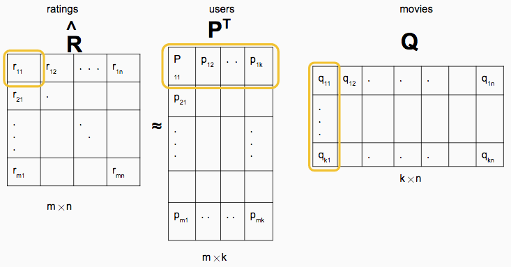
The columns of the resulting matrices \(P\) and \(Q\) turn out to contain columns with \(k\) latent features about the users and movies, respectively. The \(P\) and \(Q\) matrices are calculated iteratively, by fixing one and solving for the other, then repeating while alternating which one is fixed. As a side note, in case you want to look at the paper, the notation is a little different. They use \(U\) and \(M\) instead of \(P\) and \(Q\), and \(n_u\) and \(n_m\) instead of \(m\) and \(n\). I’ll stick with the tutorial notation in this post.
The equations for solving for \(P\) and \(Q\) are quite similar, so let’s just look at the equation for \(P\). In each iteration, the column for each user in \(P\) is generated with the following equation:
\(\mathbf{p}_i = A_i^{-1} V_i\) where \(A_i = Q_{I_i} Q_{I_i}^T + \lambda n_{p_i} E\) and \(V_i = Q_{I_i} R^T(i, I_i)\)
Here, \(E\) is the \((k \times k)\) identity matrix, \(n_{p_i}\) is the number of movies rated by user \(i\), and \(I_i\) is the set of all movies rated by user \(i\). That \(I_i\) in \(Q_{I_i}\) and \(R(i, I_i)\) means we are selecting only the columns for movies rated by user \(i\), and the way that selection is made makes all the difference.
Selecting Columns
In the tutorial, the key lines to generate each \(\mathbf{p}_i\) look like this:
Ai = np.dot(Q, np.dot(np.diag(Ii), Q.T)) + lmbda * nui * E
Vi = np.dot(Q, np.dot(np.diag(Ii), R[i].T))
P[:,i] = np.linalg.solve(Ai,Vi)
Notice that in the equation for \(A_i\), the way it removes columns for movies that weren’t reviewed by user \(i\) is creating a \((n \times n)\) matrix with the elements of \(I_i\) along the diagonal, then doing a \((n \times n) \times (n \times k)\) matrix multiplication between that and \(Q^T\), which zeroes out columns of \(Q\) for movies user \(i\) did not review. This matrix multiplication is an expensive operation that (naively) has a complexity of \(O(kn^2)\) (although probably a bit better with the numpy implementation). A similar operation is done in the \(V_i\) calculation. Even though this is not as expensive (complexity of \(O(n^2)\)), that’s still an operation we’d like to avoid if possible.
On reading the equations and Matlab algorithm implementation in the original paper, I noticed that rather than zeroing out unwanted columns, they actually remove those columns by creating a submatrix of \(Q\) and a subvector of \(\mathbf{r}_i\). This does 2 important things: First, it lets us remove that inner matrix multiplications. Second, it dramatically reduces the cost of the remaining matrix multiplications. Since we have a density of only about 6% in our \(R\) matrix, the cost of both \(Q_{I_i}Q_{I_i}^T\) and \(Q_{I_i}R^T(i,I_i)\) should theoretically be reduced to about 6% of their original costs, since the complexities of those operations (\(O(nk^2)\) and \(O(nk)\)) are both linearly dependent on \(n\). Here’s the code that replaces the 3 lines shown above:
# Get array of nonzero indices in row Ii
Ii_nonzero = np.nonzero(Ii)[0]
# Select subset of Q associated with movies reviewed by user i
Q_Ii = Q[:, Ii_nonzero]
# Select subset of row R_i associated with movies reviewed by user i
R_Ii = R[i, Ii_nonzero]
Ai = np.dot(Q_Ii, Q_Ii.T) + lmbda * nui * E
Vi = np.dot(Q_Ii, R_Ii.T)
P[:, i] = np.linalg.solve(Ai, Vi)
By making that replacement and a similar one for the equations for \(\mathbf{q}_j\), a series of 15 iterations went from taking 15-16 minutes down to about 13 seconds: a ~70-fold speedup! Check out the notebook with my updates on GitHub, or clone the whole repo to run it yourself.
Conclusions
The moral of the story here is that sometimes things that don’t seem like a big deal at first glance can make huge changes in the performance of your algorithms. This exercise reinforced in my mind the value of spending a little extra time to make sure you understand the algorithm or tool you’re using. And more specifically, if you have a sparse dataset, make that sparsity work for you.